Public safety radio communications, like all other radio communications, rely on the atmosphere as the medium over which the signals are "carried" from the transmitter to the receiver. As a result, the quality of the communications is dependent on the physical factors that influence the propagation of electromagnetic (EM) signals in this medium. The intent of this topic is to acquaint readers with the basic precepts of radio frequency signal propagation and to provide an appreciation for the effects that frequency of operation and separation distance between the radios have on the propagation characteristics and the quality of communications. This understanding is important for system specification and equipment procurement. At the same time, the reasons why some frequency bands are considered the "beach front property" of the EM spectrum are highlighted.
Electromagnetic energy typically radiates from an antenna to a distant station in four ways as shown in the diagram below. These ways are the direct, or line of sight (LOS) wave, the sky wave, the ground-reflected wave, and the surface wave. By far, the most dominant mode is the direct wave; however, the other modes may have a significant impact on the resultant received signal. 1

In addition, the electromagnetic waves coming from the antenna experience three other phenomena; reflection, diffraction, and scattering. Reflection occurs when the electromagnetic signal, or wave, reflects off an object such as the ground, water, or a building similar to how light reflects off objects. Diffraction of the signal occurs when the signal "bends" around objects such as hilltops. Finally, scattering occurs when the signal encounters objects that are much smaller in size than the wavelength of the signal and as a result the signal is dispersed in many directions such as when a signal impinges on foliage, trees, rough surfaces, etc. All of these factors affect the transmitted signal as it is "carried" through the air medium to the distant receiving antenna.
In general, radio communications between two points (the transmit radio and the receive radio; and vice versa of course if the communications are both ways!) are characterized by a "link budget." This budget is an allocation of the available power and an accounting for all of the gains and losses in power between the transmitter and the receiver. All receivers have a minimum acceptable average signal power that must be received in order to ensure proper demodulation and decoding of the transmitted signal for an acceptable level of performance. A typical link budget between two radios is depicted below.
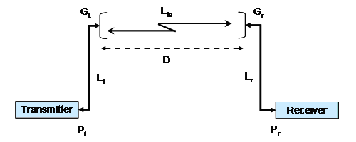
The transmit station has an average output power from the transmitter, Pt, and losses associated with cabling, connectors, couplers, etc. denoted by Lt. The transmit antenna has a characteristic gain (output power is greater than the input power to the antenna), Gt, that is dependent on the geometry of the antenna and the wavelength of the signals being transmitted. Similarly at the receiver, the antenna has gain, Gr, and sundry losses, Lr, associated with cabling, coupling, etc. At the "front end" of the receiver, the received signal is presented to the receiver itself for processing. It is critical for the received power level, Pr, to be sufficient to meet the performance requirements of the radio.
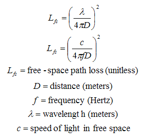
If the antenna at the transmitter is considered a point source of energy, then the electromagnetic energy will radiate away from the antenna in all directions in an equal manner and the antenna may be considered as an "isotropic" source. In which case, the energy radiated from the antenna will dissipate strictly by free space dispersion. As the signal radiates away from the antenna, it will lose energy as the EM wave scatters away from the antenna. This "free space path loss," denoted by Lfs, will be the dominant factor in the loss of signal energy as the transmitted signal moves away from the antenna.
This loss is dependent on the spherical geometry of the space around the point source antenna, the frequency of the signal being transmitted, and the distance from the source antenna. This relationship is given by;
By Friis' formula, the ratio of the received signal power to the transmitted signal power is given by the relationship:2
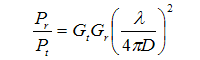
This expression accounts for the free space path loss and the antenna gains, Gt and Gr, to simply give an overall relationship between the transmitted power, Pt, and the received power, Pr, as a function of the distance, D, between the antennas and the wavelength (frequency3) of the transmitted signal. It should be noted that this relationship assumes a direct "line of sight" between the two antennas. There are of course many different paths that the transmitted electromagnetic signal may take between the transmit and receive antennas, but the direct path between the two is the most dominant. Thus, the fundamental relationship of Friis' formula between the transmitted signal power, the gains of the two antennas and the dominant free space path loss gives the resulting received signal power at the distant receiver.4
By converting Friis' formula to logarithmic terms, we convert the relationship to simply an algebraic expression in decibels.5 Hence,

First, let us examine the import of frequency and distance in the free space path loss term of Frii's expression. The table below is a compilation of the free space path loss for various frequencies that are of interest to public safety users and the distances are typical ranges between user terminals.
| Distance (Miles) | Frequency (MHz) | Path Loss (dB) |
|---|---|---|
| 10 | 150 | 100.095 |
| 10 | 450 | 109.637 |
| 10 | 770 | 114.303 |
| 10 | 850 | 115.161 |
| 10 | 1725 | 121.309 |
| 20 | 150 | 106.115 |
| 20 | 450 | 115.658 |
| 20 | 770 | 120.323 |
| 20 | 850 | 121.182 |
| 20 | 1725 | 127.329 |
| 30 | 150 | 109.637 |
| 30 | 450 | 119.180 |
| 30 | 770 | 123.845 |
| 30 | 850 | 124.704 |
| 30 | 1725 | 130.851 |
| 50 | 150 | 114.074 |
| 50 | 450 | 123.617 |
| 50 | 770 | 128.282 |
| 50 | 850 | 129.141 |
| 50 | 1725 | 135.288 |
This table reflects two very important propagation characteristics. First, for a given frequency the path loss increases with increased distance. In the examples cited, for a frequency of 450 MHz, the path loss increases from 109.64 dB at 10 miles to 123.62 dB at 50 miles. This difference of 14 dB can have a significant impact on the quality of the received signal. Notice that for a factor of two increase in distance, the loss increases by 6 dB; again, this is characteristic of the path loss formula. It should also be noted at this point that there is a commonly used expression resulting from the path loss formula above that the free space path loss increases with the square of the distance between the two terminals.
The second important observation is that for a given distance the path loss increases with increased frequency. Looking at the losses for 30 miles for example, the path loss increases from 109.64 dB at 150 MHz to 130.85 dB at 1725 MHz. Again, the 21 dB difference could have a potentially significant and detrimental impact on communications. Also, it should be noted that a factor of two increase in frequency will result in a 6 dB increase in the loss for the constant distance. As another expression, path loss increases with the square of the increase in frequency.
The import of the free space path loss on a radio link can now be illustrated. Typical values of some of the parameters for current public safety equipment6 can be used to show the import of free space path loss along with the impact that frequency and distance have on the propagation process. Assume that the transmitting station is a base station with 50 Watts average transmit power; cabling, etc., losses of 2 dBi, antenna gain of 7 dBi, and the receive station is a hand-held receiver with antenna gain of 3 dBi plus cabling losses of 2 dBi. Furthermore, assume that the transmit signal frequency is in the public safety bands as shown in the table above for the distances shown above. Also assume that the mobile receiver has a sensitivity of -119 dBm.7 Combining these parameters and factors, we obtain the following results for the down-link budget from base station to mobile station.
For Pt = 50 W, Lt=Lr = 2 dBi, Gt =7 dBi, Gr = 3 dBi, Rcvr Sensitivity = -119 dBm;
| Distance (Miles) | Frequency (MHz) | Path Loss (dB) | Power Rcvd (dBm) | Margin (dBm) |
|---|---|---|---|---|
| 10 | 150 | 100.095 | -47.105 | 71.895 |
| 10 | 450 | 109.637 | -56.647 | 62.353 |
| 10 | 770 | 114.303 | -61.313 | 57.687 |
| 10 | 850 | 115.161 | -62.172 | 56.828 |
| 10 | 1725 | 121.309 | -68.319 | 50.681 |
| 20 | 150 | 106.115 | -53.126 | 65.874 |
| 20 | 450 | 115.658 | -62.668 | 56.332 |
| 20 | 770 | 120.323 | -67.334 | 51.666 |
| 20 | 850 | 121.182 | -68.192 | 50.808 |
| 20 | 1725 | 127.329 | -74.340 | 44.660 |
| 30 | 150 | 109.637 | -56.647 | 62.353 |
| 30 | 450 | 119.180 | -66.190 | 52.810 |
| 30 | 770 | 123.845 | -70.855 | 48.145 |
| 30 | 850 | 124.704 | -71.714 | 47.286 |
| 30 | 1725 | 130.851 | -77.861 | 41.139 |
| 50 | 150 | 114.074 | -61.084 | 57.916 |
| 50 | 450 | 123.617 | -70.627 | 48.373 |
| 50 | 770 | 128.282 | -75.292 | 43.708 |
| 50 | 850 | 129.141 | -76.151 | 42.849 |
| 50 | 1725 | 135.288 | -82.298 | 36.702 |
Analysis of this link budget reveals several important results. First, as suggested above both frequency and separation distance affect the radio link performance. The column designated as the "Margin" is the difference between the received power and the sensitivity of the receiver radio. It is a reflection of the amount of received signal power that may fluctuate due to dynamic changes in the signal propagation without affecting the performance of the receiver. The table shows that, as distance from the transmitter increases, the available margin in operating power declines, suggesting that as the receiver is farther from the transmitter then the dynamics of radio signal propagation will have more effect on the radio link performance. This degradation in performance with increased distance is very intuitive - recall our comment earlier regarding the path loss being dependent on the square of the distance.
This table also reflects a similar analysis based on frequency such that for a given distance as the frequency increases then the operating margin is reduced. This degradation in performance due to a higher operating frequency is not as intuitive as the distance relationship, but in a similar manner, the path losses increase in a squared relationship to the frequency. The result in either case is a reduced margin for satisfactory performance.
In the example provided above, the operating margins are pretty significant and should allow for good performance, but this performance is based on a strong signal from the base station to the mobile receiver. By reversing the situation and doing a link budget from the mobile station to the base station, a very different situation emerges. The typical transmit power of a mobile station is 5 Watts. Assuming the other parameters remain the same (since the antennas, cabling, and free space loss are reciprocal, i.e. same values in both directions!), then the "uplink" budget is as follows.
For Pt = 5 W, Lt=Lr = 2 dBi, Gt =3 dBi, Gr = 7 dBi, Rcvr Sensitivity = -119 dBm;
| Distance (Miles) | Frequency (MHz) | Path Loss (dB) | Power Rcvd (dBm) | Margin (dBm) |
|---|---|---|---|---|
| 10 | 150 | 100.095 | -57.105 | 61.895 |
| 10 | 450 | 109.637 | -66.647 | 52.353 |
| 10 | 770 | 114.303 | -71.313 | 47.687 |
| 10 | 850 | 115.161 | -72.172 | 46.828 |
| 10 | 1725 | 121.309 | -78.319 | 40.681 |
| 20 | 150 | 106.115 | -63.126 | 55.874 |
| 20 | 450 | 115.658 | -72.668 | 46.332 |
| 20 | 770 | 120.323 | -77.334 | 41.666 |
| 20 | 850 | 121.182 | -78.192 | 40.808 |
| 20 | 1725 | 127.329 | -84.340 | 34.660 |
| 30 | 150 | 109.637 | -66.647 | 52.353 |
| 30 | 450 | 119.180 | -76.190 | 42.810 |
| 30 | 770 | 123.845 | -80.855 | 38.145 |
| 30 | 850 | 124.704 | -81.714 | 37.286 |
| 30 | 1725 | 130.851 | -87.861 | 31.139 |
| 50 | 150 | 114.074 | -71.084 | 47.916 |
| 50 | 450 | 123.617 | -80.627 | 38.373 |
| 50 | 770 | 128.282 | -85.292 | 33.708 |
| 50 | 850 | 129.141 | -86.151 | 32.849 |
| 50 | 1725 | 135.288 | -92.298 | 26.702 |
Review of the results at a close distance of 10 miles shows the typical decrease in margin with higher operating frequency but the operating margins are still significant enough that any dynamics in propagation losses will not have a large impact on performance. At larger distances on the other hand, we see the reduced margins that result from distance and increases in frequency so that any dynamical changes in losses could have an impact on performance. It should be intuitive that the smaller transmitter power would limit the range; and now we see that frequency also has an impact on the radio system performance.
Now it is necessary to introduce two other factors that influence the free space path loss of electromagnetic signals. Unfortunately, pure physics comes into play when the frequency of transmitted signals increases beyond 10 GHz. The two factors that influence propagation of signals above 10 GHz are oxygen molecules in the air and water molecules that are in the air.8 Both molecular structures absorb energy depending on the frequency of the EM signal and cause increased path loss for the signals. The impact of these two factors is shown in the loss chart below, which shows the free space path loss (attenuation) as a function of frequency.9
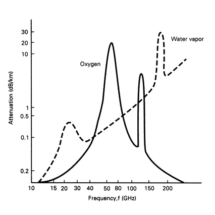
The reasons for suggesting that certain frequency bands are "beach front property" become a bit more obvious at this point. First, the bands below 10 GHz do not suffer from the attenuation due to water or oxygen as well as the increased losses due to scattering at higher frequencies. Second, for frequency bands in the HF (3-30 MHz) and VHF (30-300 MHz) ranges and below, the number of potential channels and the potential channel bandwidths are more limited. The result is that the frequency bands in the UHF (300-3000 MHz) range are prime locations for mobile services. It is for these reasons that the UHF frequency bands - especially the allocations in the 700 MHz and 800 MHz bands - are particularly attractive for mobile commercial and public safety services. Hence, these bands are considered "prime real estate" in the magnetic spectrum.
As suggested earlier in this topic, signals being sent from a transmitter to a distant receiver may experience any number of disruptions due to their particular path such as reflections off large objects (buildings, etc.), diffraction around or over objects, and scattering due to impinging on smaller objects. These factors have been accounted for by a number of researchers who have defined a number of empirical formulas for path loss that account for all of these factors. These practical path loss formulas are based strictly on measured data and empirical formulation. The formulas are used frequently now to account for all losses and predict the overall path loss in specific applications. The models include the following:
- Longley-Rice Model 10 (Also known as the Irregular Terrain Model, ITM)
- Edwards-Durkin Model 11
- Okumura Model 12
- Hata Model 13
- Cost-231 Model 14
- Walfisch and Bertoni Model 15
- Cost-231 Walfisch and Ikegami Model 16
There are also a number of models that have been formulated to account for losses inside buildings and other structures as well as models that account for fading affects and the Doppler affects that result from movement on the part of the radio terminals. 17
It is extremely important at this point to make the connection between these empirical models and the aforementioned free space path loss predictions and link budgets. As shown by Rappaport for example,18 the simplistic Okumura model predicts that the correction factor for loss above the median attenuation (free space loss) at 450 MHz will vary between 25-50 dB depending in distance!! If this additional path loss is added to the projected link budgets, then for the base station transmit link budget, the receiver margins are reduced to the point that communications at 50 miles would become problematic and variable. Even more importantly, the additional loss applied to the mobile transmit budget would RULE OUT communications at 50 miles, have a significant impact at 30 miles, and most likely even have an effect on communications as close as 20 miles! Therefore, it is important to understand the impact of frequency and distance on the quality of communications and for communications planning.
In summary, this topic addressed the primary factors affecting the transmission of radio signals. In particular, the deleterious impacts of increasing signal frequency and increasing distance between transmitter and receiver as factors in signal propagation were illustrated. This topic focused on the impact of free space path loss which is inherent in the natural propagation of electromagnetic signals away from an antenna. The analysis assumed direct line of sight between the two radios and considered only the primary impact of free space path loss. In reality, the propagation of signals is much more complicated due to physical objects such as buildings, refraction of the signals around physical objects, scattering due to foliage, etc. and many other factors that also include the results of motion that cause Doppler spreading of the signals. Thus, it is important for public safety entities to recognize the importance that these physical parameters will have on the performance of their radio systems and how they must engineer their equipment and systems to meet their communications requirements.
1 Wayne Tomasi, Electronic Communications Systems, Fundamentals Through Advanced, 4th Edition, Prentice-Hall, Upper Saddle River, NJ, 2001, p. 359.
2 Friis, H.T., "A Note on a Simple Transmission Formula," Proceedings of the IRE, Vol. 34, May 1946, p. 254.
3 Wavelength, λ, and frequency, f, are related by the constant of the speed of light, c; such that λ = c / f where the speed of light is given as 3x10⁸ meters per second, the frequency is in Hertz (cycles per second), and the resulting wavelength is in meters.
4 It should also be noted that the transmit power may be expressed in either dBW, a decibel power corresponding to an average transmit power in Watts, or in dBm, a decibel power corresponding to an average transmit power in milliwatts. The antenna gains and cabling losses are reflected in dBi corresponding to the isotropic antenna as opposed to dBd for half-wave dipole antennas. If dBd were used instead, there would be a difference (less) of 2.15 dB since there is a gain of 1.65 (power ratio) when comparing isotropic antennas to half-wave dipole antennas. A dipole antenna has a gain of 1.65 (2.15 dB) above an isotropic. To complete the thought, the product of PtGt represents the average transmit power times the antenna gain and is referred to as isotropic if the antenna is considered a point source (such that all relationships are considered in the far field). Hence, this is called the effective isotropic radiated power or EIRP. When this combination is referenced to a half-wave dipole then the radiated power is called the effective radiated power or ERP.
5 By definition, 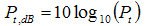
6 All of the typical transmitter, receiver, and antenna parameters are taken from the "Specs Guide 2009" published in Mission Critical Magazine, Vol. 24, No.1, January 2009.
7 Sensitivity is a measure of the minimum signal power that the receiver must have to successfully decipher, demodulate, and process the received signal for use by the intended user.
8 See FCC Office of Engineering and Technology Bulletin Number 70, July 1997, "Millimeter Wave Propagation: Spectrum Management Implications," at https://www.fcc.gov/oet/info/documents/bulletins/.
9 Tomasi, p. 352.
10 Rice, P.L., Longley, A.G., Norton, K.A., and Barsis, A.P., "Transmission Loss Predictions for Tropospheric Communications Circuits," National Bureau of Standards Technical Note 101; Volumes I and II; issued May 7, 1965; revised May 1, 1966; revised January 1967. This model is the basis for a number of FCC Rules - for example, see https://www.fcc.gov/oet/info/documents/bulletins/ - including the radio and television broadcast rules.
11 Edwards, R., and Durkin, J., "Computer Prediction of Service Area for VHF Mobile Radio Networks," Proceedings of the IEE, Vol. 116, No. 9, pp. 1493-1500, September 1969.
12 Okumura, T., Ohmori, E., and Fukeda, K., "Field Strength and Its Variability in VHF and UHF Land Mobile Service," Review Electrical Communication Laboratory, Vol. 16, No. 9-10, pp. 825-873, September-October 1968.
13 Hata, Masaharu, "Empirical Formula for Propagation Loss in Land Mobile Radio Services," IEEE Transactions on Vehicular Technology, Vol. VT-29, No. 3, pp. 317-325, August 1980. The Hata model extended the Okumura model to empirically derive correction factors for city and suburban environments. See http://ieeexplore.ieee.org/stamp/stamp.jsp?arnumber=1622772&isnumber=34048.
14 The European Co-operative for Scientific and Technical Research (EURO-COST) formed the COST-231 model to extend the Hata-Okumura model to 2 GHz. See reference at; European Cooperation in the Field of Scientific and Technical Research EURO-COST 231, "Urban Transmission Loss Models for Mobile Radio in the 900 and 1800 MHz Bands," Revision 2, The Hague, September, 1991.
15 Walfisch, J. and Bertoni, H.L., "A Theoretical Model of UHF Propagation in Urban Environments," IEEE Transactions on Antennas and Propagation, Vol. AP-36, pp. 1788-1796, October 1988.
16 Ikegami, F., Takeuchi, T., and Yoshida, S., "Theoretical Prediction of Mean Field Strength for Urban Mobile Radio," IEEE Transactions on Antennas and Propagation, Vol.39, No.3, 1991, and see http://www.cse.hcmut.edu.vn/~ltquan/Documents_Softwares/CDMA/Walfisch-Ikegami.htm.
17 For more information on the characterization of propagating signals and potential interference, see the Telecommunications Industry Association web site at http://www.tiaonline.org/index.cfm and in particular http://network.tiaonline.org/2008/May14/standards_update.cfm#TSB for TIA Bulletin TSB-88.1-C, Wireless Communications Systems Performance in Noise-Limited Situations, Part 1: Recommended Methods for Technology-Independent Performance Modeling. TSB-88.1-C supersedes TSB-88-B (including addendum TSB-88-B1). In addition, see TIA Bulletin TSB 10-F (Interference Criteria for Microwave Systems). Also, the National Institute of Standards (NIST) maintains a bibliography of wireless propagation studies at http://w3.antd.nist.gov/wctg/manet/wirelesspropagation_bibliog.html.
18 Theodore S. Rappaport, Wireless Communications Principles and Practice, Upper Saddle River, NJ; Prentice-Hall PTR, July 1996.